
Website owner: James Miller
Small sampling theory. Student’s t distribution. The chi-square distribution. Confidence intervals. Tests of hypotheses and significance.
Small sampling theory. A study of sampling distributions of statistics employing small samples is called small sampling theory. A more suitable name, however, would be exact sampling theory since the results obtained hold for large as well as small samples. By a small sample we mean a sample of size n < 30.
Two important distributions used for the case of small samples is the Student’s t distribution and the chi-square distribution.
Student’s t distribution. Let us first define the statistic

which is analogous to the statistic given by

Here:
![]()
s — sample standard deviation
n — sample size
μ and σ — population mean and standard deviation
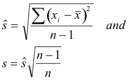
![]() is the modified standard deviation where
is the modified standard deviation where

If we consider samples of size n drawn from a normal (or
approximately normal) population with mean μ and if for
each sample we compute t, using the sample mean
![]() and the
sample standard deviation s or
and the
sample standard deviation s or
![]() , the sampling distribution
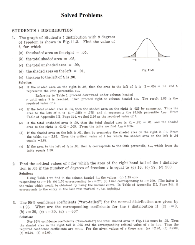
for t can be obtained. This distribution (see Fig. 1), called the
Students’s t distribution, is given by
, the sampling distribution
for t can be obtained. This distribution (see Fig. 1), called the
Students’s t distribution, is given by

where Y0 is a constant depending on n such that the total area under the curve is one and the constant ν = n -1 is called the number of degrees of freedom. (The definition of degrees of freedom will be given later.)
Let us now go over the above computational process step by step in more detail.
1. We take m samples, each of sample size n
2. On each sample we compute the sample mean
![]() , the sample standard deviation s, and the
value of t from the formula
, the sample standard deviation s, and the
value of t from the formula
![]()
using the sample mean
![]() as an approximation for the population mean μ.
as an approximation for the population mean μ.
For large m the values of t will follow Student’s t distribution 2).
This distribution is named after its discoverer Gosset, who published his works under the pseudonym “Student” during the early part of the twentieth century.
For large values of ν or n (certainly n > 30) the curves closely approximate the standardized normal curve

as shown in Fig. 1.
Percentile. A value on a scale of 100 that indicates the percent of a distribution that is equal to or below it. It is a way of expressing where an observation falls in a range of other observations. For example, if a score falls in the 20th percentile, this means that 20 percent of all the scores recorded are lower.
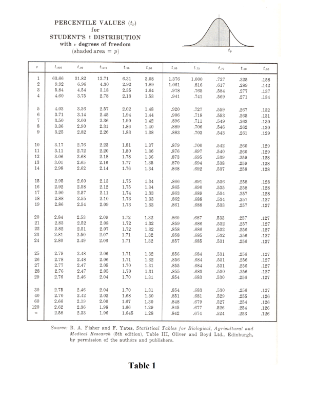
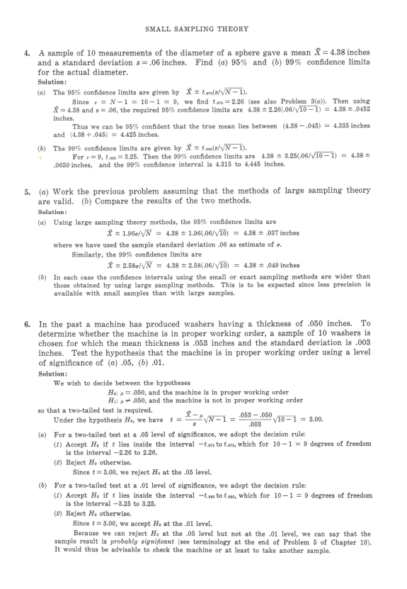
Confidence intervals. We can define 95%, 99% or other confidence intervals by using the table of the t distribution. See Table 1.
For example, if -t.975 and t.975 are the values of t for which 2.5% of the area lies in each “tail” of the t distribution, then a 95% confidence interval for t is
![]()
With some algebraic manipulation we obtain

from which we see that μ is estimated to lie in the interval given by 4) with 95% confidence (i.e. probability .95). Note that t.975 represents the 97.5 percentile value, while -t.975 = -t.975 represents the 2.5 percentile value.
In general, we can represent confidence limits for population means by

where the values +tc, called critical values or confidence limits, depend on the level of confidence
desired and the sample size. They can be read from Table 1.
Tests of hypotheses and significance. The tests of hypotheses and significance used for large samples are easily extended to problems involving small samples, the only difference being that the z score or z statistic is replaced by a suitable t score or t statistic.
1. Means
To test the hypothesis H0 that a normal population has mean μ, we use the t score or t statistic
![]()
where
![]() is the mean of a sample of size n.
is the mean of a sample of size n.
This is analogous to using the z score,

for large n except that
![]()
is used in place of σ. The difference is that while z is normally distributed, t follows Student’s distribution. As n increase, these tend toward agreement.
2. Differences of Means
Suppose that two random samples of sizes n1 and n2 are drawn from normal populations whose
standard deviations are equal (σ1 = σ2). Suppose further that these two populations have means
and standard deviations given by
![]() respectively. To test the hypothesis H0 that the
samples come from the same population (i.e. μ1 = μ2, as well as σ1 = σ2) we use the t score given
by
respectively. To test the hypothesis H0 that the
samples come from the same population (i.e. μ1 = μ2, as well as σ1 = σ2) we use the t score given
by

The distribution of t is Student’s distribution with ν = n1 + n2 - 2 degrees of freedom.
The chi-square distribution.
Here:
![]()
s — sample standard deviation
n — sample size
μ and σ — population mean and standard deviation
Let us define the statistic

where χ is the Greek letter chi and is read chi-square.
If we consider samples of size n drawn from a normal population with a standard deviation σ, and if for each sample we compute χ2 , a sampling distribution for χ2 can be obtained. This distribution, called the chi-square distribution, is given by
![]()
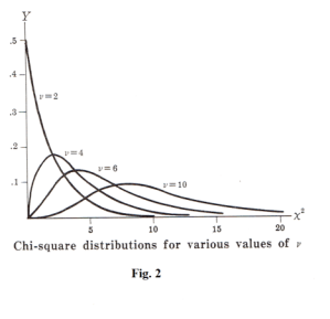
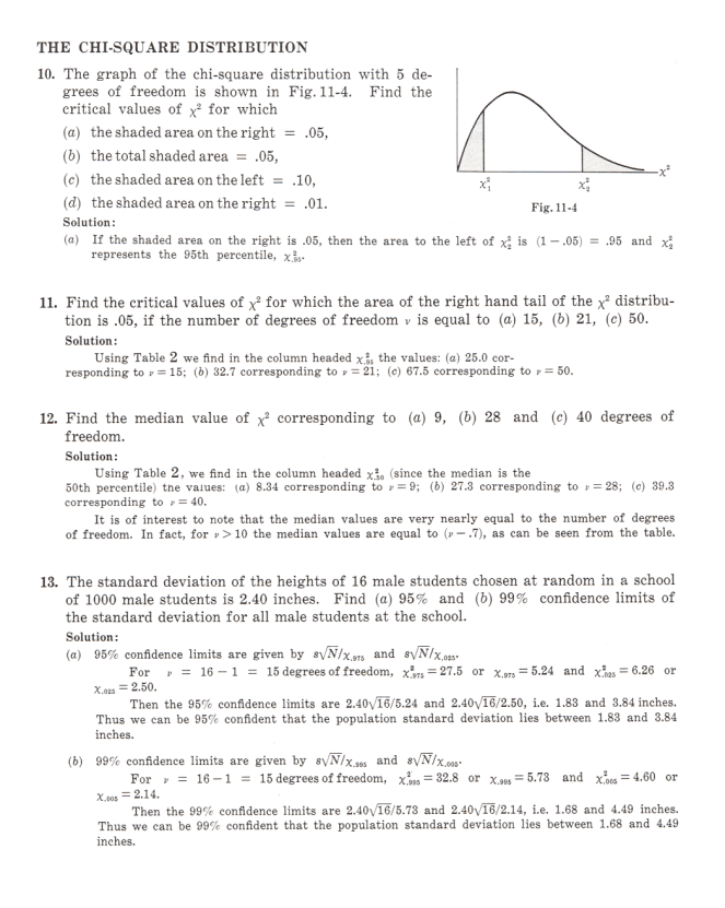
where ν = n - 1 is the number of degrees of freedom, and Y0 is a constant depending on ν such that the total area under the curve is one. The chi-square distributions corresponding to various values of ν are shown in Fig. 2.
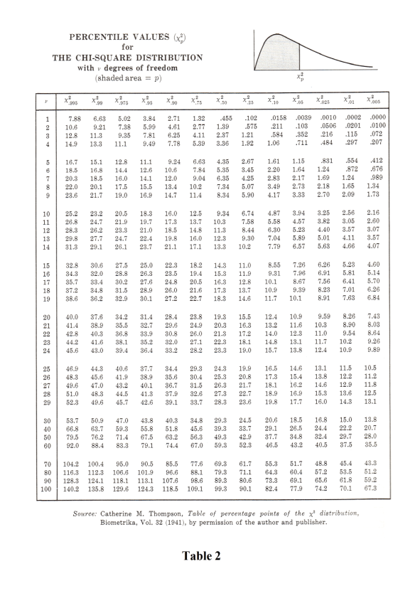
Confidence intervals for χ2. As is done with the normal and t distributions, we can define 95%, 99% or other confidence limits and intervals for χ2 by use of the table of the χ2 distribution. See Table. 2. In this manner we can estimate within specified limits of confidence the population standard deviation σ in terms of the a sample standard deviation s.
For example, if
![]() and
and
![]() are the values of χ2 (called critical values) for which 2.5% of the
area in each “tail” of the distribution, then the 95% confidence interval is
are the values of χ2 (called critical values) for which 2.5% of the
area in each “tail” of the distribution, then the 95% confidence interval is

With some algebraic manipulation we obtain

Thus σ is estimated to lie in the interval indicated with 95% confidence. Similarly other
confidence intervals can be found. The values
![]() and
and
![]() represent respectively the 2.5 and
97.5 percentile values.
represent respectively the 2.5 and
97.5 percentile values.
Table 2 gives percentile values corresponding to the number of degrees of freedom ν.
Degrees of freedom. In order to compute a statistic such as 1) or 8), it is necessary to use observations obtained from a sample as well as certain other parameters. If these parameters are unknown they must be estimated from a sample.
The number of degrees of freedom of a statistic generally denoted by ν is defined as the number n of independent observations in the sample (i.e. the sample size) minus the number k of population parameters which must be estimated from sample observations. In symbols, ν = n - k.
In the case of the statistic 1) the number of independent observations in the sample is n, from
which we can compute
![]() and s. However, since we must estimate ν, k = 1 and so ν = n - 1.
and s. However, since we must estimate ν, k = 1 and so ν = n - 1.
In the case of the statistic 8) the number of independent observations in the sample is n, from
which we can compute
![]() and s. However, since we must estimate σ, k = 1 and so ν = n - 1.
and s. However, since we must estimate σ, k = 1 and so ν = n - 1.
Portions, examples, solved problems excerpted from Murray R. Spiegel. Statistics. Schaum.
References
Murray R Spiegel. Statistics (Schaum Publishing Co.)
Jesus Christ and His Teachings
Way of enlightenment, wisdom, and understanding
America, a corrupt, depraved, shameless country
On integrity and the lack of it
The test of a person's Christianity is what he is
Ninety five percent of the problems that most people have come from personal foolishness
Liberalism, socialism and the modern welfare state
The desire to harm, a motivation for conduct
On Self-sufficient Country Living, Homesteading
Topically Arranged Proverbs, Precepts, Quotations. Common Sayings. Poor Richard's Almanac.
Theory on the Formation of Character
People are like radio tuners --- they pick out and listen to one wavelength and ignore the rest
Cause of Character Traits --- According to Aristotle
We are what we eat --- living under the discipline of a diet
Avoiding problems and trouble in life
Role of habit in formation of character
Personal attributes of the true Christian
What determines a person's character?
Love of God and love of virtue are closely united
Intellectual disparities among people and the power in good habits
Tools of Satan. Tactics and Tricks used by the Devil.
The Natural Way -- The Unnatural Way
Wisdom, Reason and Virtue are closely related
Knowledge is one thing, wisdom is another
My views on Christianity in America
The most important thing in life is understanding
We are all examples --- for good or for bad
Television --- spiritual poison
The Prime Mover that decides "What We Are"
Where do our outlooks, attitudes and values come from?
Sin is serious business. The punishment for it is real. Hell is real.
Self-imposed discipline and regimentation
Achieving happiness in life --- a matter of the right strategies
Self-control, self-restraint, self-discipline basic to so much in life