Statistical decisions. Statistical hypotheses. Null hypotheses. Tests of hypotheses and significance. Type I and Type II errors. Level of significance. Tests involving the normal distribution. One-tailed and two-tailed tests. Operating characteristic curves. Control Charts.

SolitaryRoad.com

Website owner:  James Miller

[ Home ] [ Up ] [ Info ] [ Mail ]

Statistical decisions. Often in practice we are called to make decisions about populations on the basis of sample information. Such decisions are called statistical decisions. For example, one might wish to decide on the basis of some sample data whether a new serum is really effective in curing a disease, whether one educational procedure is better than another, whether a given coin is loaded, etc.

Statistical hypotheses. Null hypotheses. In attempting to reach decisions, it is useful to make assumptions or guesses about the populations involved. Such assumptions, which may or may not be true, are called statistical hypotheses and in general are statements about the probability distributions of the populations.

In many instances we formulate a statistical hypothesis for the sole purpose of rejecting or nullifying it. For example, if we want to decide whether a given coin is loaded we formulate the hypothesis that the coin is fair, i.e. p = .5, where p is the probability of heads. Similarly, if we want to decide whether one procedure is better than another, we formulate the hypothesis that there is no difference between the procedures (i.e. any observed differences are merely due to fluctuations in sampling in the same population). Such hypotheses are often called null hypotheses and are denoted by H₀.

Any hypothesis which differs form a given hypothesis is called an alternative hypothesis. For example, if one hypothesis is p =.5, alternative hypotheses are p = .7, p ≠ .5. or p ≥ .5. A hypothesis alternative to the null hypothesis is denoted by H₁.

Tests of hypotheses and significance. If on the supposition that a particular hypothesis is true we find that results observed in a random sample differ markedly form those expected under the hypothesis on the basis of pure chance using sampling theory, we would say that the observed differences are significant and we would be inclined to reject the hypothesis (or at least not accept it on the basis of the evidence obtained). For example, if 20 tosses of a coin yield 16 heads we would be inclined to reject the hypothesis that the coin is fair, although it is conceivable that we might be wrong.

Procedures which enable us to decide whether to accept or reject hypotheses or to determine whether observed samples differ significantly form expected results are called tests of hypotheses, tests of significance, or rules of decision.

Type I and Type II errors. The test of a hypothesis has the possibility of two types of errors: 1) the rejection of the stated hypothesis when it is actually true, and 2) the acceptance of the stated hypothesis when it is actually false. If we reject the stated null hypothesis H₀ when it is actually true, we say a Type I error has been made. If we accept it when it is actually false, we say a Type II error has been made. Thus:

H₀ is true 1) accept H₀ 2) reject H₀ (Type I error)

H₀ is false 1) accept H₀ (Type II error) 2) reject H₀

In either case, whether we make a Type 1 or Type 2 error, a wrong decision or error in judgement has occurred.

In order for any tests of hypothesis or rules of decision to be good, they must be designed so as to minimize errors of decision. This is not a simple matter since, for a given sample size, an attempt to decrease one type of error is accompanied in general by an increase in the other type of error. In practice one type of error may be more serious than the other, and so a compromise should be reached in favor of a limitation of the more serious type. The only way to reduce both types of error is to increase the sample size, which may or may not be possible.

Level of significance. In testing a given hypothesis, the maximum probability with which we would be willing to risk a Type I error is called the level of significance of the test. This probability, often denoted by α, is generally specified before any samples are drawn, so that the results will not influence our choice.

In practice a level of significance of .05 or .01 is customary, although other values are used. If for example a .05 or .01 level of significance is chosen in designing a test of hypothesis, then there about 5 chances in 100 that we would reject the hypothesis when it should be accepted, i.e. we are about 95% confident that we have made the right decision. In such case we say the hypothesis has been rejected at a .05 level of significance, which means that we could be wrong with a probability .05.

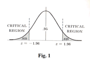
Tests involving the normal distribution. To illustrate the ideas presented above, suppose that under a given hypothesis the sampling distribution of a statistic S is a normal distribution with a mean μ_s and standard deviation σ_s. Then the distribution of the standardized variable (or z score), given by z = (S - μ_s)/σ_s, is the standardized normal distribution (mean 0, variance 1) and is shown in Fig. 1.

As indicated in the figure we can be 95% confident that, if the hypothesis is true, the z score of an actual sample statistic S will lie between -1.96 and 1.96 (since the area under the normal curve between these values is .95).

However, if on choosing a single sample at random we find that the z score of its statistic lies outside the range -1.96 to 1.96, we would conclude that such an event could happen with probability of only .05 (total shaded area in the figure) if the given hypothesis were true. We would then say this z score differed significantly form what would be expected under the hypothesis and would be inclined to reject the hypothesis.

The total shaded area .05 is the level of significance of the test. It represents the probability of our being wrong in rejecting the hypothesis, i.e. the probability of making a Type I error. Ths we say that the hypothesis is rejected at a .05 level of significance or that the z score of the given sample statistic is significant at a .05 level of significance.

The set of z scores outside the range -1.96 to 1.96 constitutes what is called the critical region or region of rejection of the hypothesis or the region of significance. The set of z scores inside the range -1.96 to 1.96 could then be called the region of acceptance of the hypothesis or the region of non-significance.

On the basis of the above remarks we can formulate the following rule of decision or test of hypothesis or significance.

(a) Reject the hypothesis at a .05 level of significance if the z score of the statistic S lies outside the range -1.96 to 1.96 (i.e. either z > 1.96 or z < 1.96). This is equivalent to saying that the observed sample statistic is significant at the .05 level.

(b) Accept the hypothesis (or is desired make no decision at all) otherwise.

Because the z score plays such an important part in tests of hypotheses and significance, it is also called a test statistic.

It should be noted that other levels of significance could have bee used. For example, if a .01 level were used we would replace 1.96 everywhere above by 2.58 (see Table B). Table A can also be used since the sum of the level of significance and level of confidence is 100%.

One-tailed and two-tailed tests. In the above test we displayed interest in extreme values of the statistic S or its corresponding z score on both sides of the mean, i.e. in both tails of the distribution. For this reason such tests are called two-tailed tests or two-sided tests.

Often, however, we may be interested only in extreme values to one side of the mean, i.e. in one “tail” of the distribution, as for example when we are testing the hypothesis that one process is better than another (which is different from testing whether one process is better or worse than the other). Such tests are called one-tailed tests or one-sided tests. In such cases the critical region is a region to one side of the distribution, with area equal to the level of significance.

Table B, which gives critical values of z for both one-tailed and two-tailed tests at various levels of significance, will be found useful for purposes of reference. Critical values of z for other levels of significance are found by use of the table of normal curve areas.

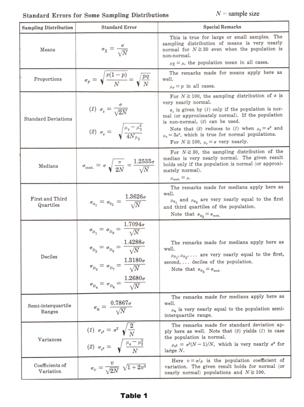
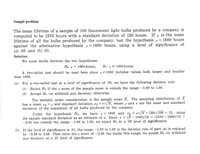
Special tests. For large samples the sampling distributions of many statistics are normal distributions (or at least nearly normal) with mean μ_s and standard deviation σ_s. In such cases we can use the above results to formulate decision rules or tests of hypotheses and significance. The following special cases taken from Table 1 are just a few of the statistics of practical interest. In each case the results hold for infinite populations or for sampling with replacement. .For sampling without replacement from finite populations the results must be modified.

1. Means.

Nomenclature

μ σ population mean and population standard deviation

sample mean and standard deviation

μ_s σ_s sampling distribution mean and standard deviation

Here S = the sample mean.

The z score is given by

where:

μ — population mean

σ — population standard deviation

n — sample size

When necessary the sample deviation s or is used to estimate σ.

2. Proportions. Here S = P, the proportion of “successes” in a sample; μ_s = μ_p = p, where p is the population proportion of successes and n is the sample size; where q = 1- p. The z score is given by

In case P = X/n, where X is the actual number of successes in a sample, the z score becomes

Results for other statistics can be similarly obtained.

Operating characteristic curves. Power of a test. We have seen how the Type I error can be limited by properly choosing a level of significance. It is possible to avoid risking Type II errors altogether by simply not making them, which amounts to never accepting hypotheses. In many practical cases, however, this cannot be done. In such cases use is often made of operating characteristic curves, or OC curves, which are graphs showing the probabilities of Type II errors under various hypotheses. These provide indications of how well given tests will enable us to minimize Type II errors, i.e. they indicate the power of a test to avoid making wrong decisions. They are useful in designing experiments by showing, for instance, what sample sizes to use.

Control Charts. It is often important in practice to know when a process has changed sufficiently so that steps may be made to remedy the situation. Such problems arise, for example, in quality control where one must, often quickly, decide whether observed changes are due simply to chance fluctuations or to actual changes in a manufacturing process because of deterioration of machine parts, mistakes of employees, etc. Control charts provide a useful and simple method for dealing with such problems.

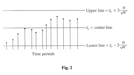
A control chart consists of three lines: a center line, an upper line and a lower line. The means of successive samples are plotted on the chart. See Fig. 2.

The center line, denoted by , represents the average of k sample means each computed from n observations. Generally we take k ≥25, n ≥4.

where x_ij is the jth observation in sample i.

The upper and lower control lines are computed from

where σ is the standard deviation of the sample means.

Nearly all sample means should fall between the lower and upper lines.

Much of the above excerpted from Murray R. Spiegel. Statistics. Schaum.

For examples, worked problems, and clarification see Theory and Problems of Statistics by Murray R. Spiegel, Schaum’s Outline Series, Schaum Publishing Co.

References

Murray R Spiegel. Statistics (Schaum Publishing Co.)